library(tidyverse)
library(knitr)14 New lm Predict Left & Predict Right
ggplot has some lovely built-in geoms that can show model extrapolations. Sometimes you might want to only show a line either before or after a certain point on an axis. This script shows how to achieve this manually.
14.1 Make new functions
First we create a pair of new functions which decorate an lm object to the right.
lm_right <- function(formula,data,...){
                                      mod <- lm(formula,data)
                                      class(mod) <- c('lm_right',class(mod))
                                      mod
                                      }
and another that decorates an lm object to the left.
  lm_left <- function(formula,data,...){
                                        mod <- lm(formula,data)
                                        class(mod) <- c('lm_left',class(mod))
                                        mod
                                        }
Then create a new function which truncates the data of a model to the right of a defined point
  predictdf.lm_right <-
    function(model, xseq, se, level){
                            init_range = range(model$model$x)
                            xseq <- xseq[xseq >=init_range[1]]
                            ggplot2:::predictdf.default(model, xseq[-length(xseq)], se, level)
                                    }
and a counterpart which does the same, but to the left
 predictdf.lm_left <-
    function(model, xseq, se, level){
                            init_range = range(model$model$x)
                            xseq <- xseq[xseq <=init_range[2]]
                            ggplot2:::predictdf.default(model, xseq[-length(xseq)], se, level)
                                    }
Now we can apply the new functions to a dummy dataset to get a feel for what they do
14.2 Dummy Data Set
The dummy data set is a simulated time series where some kind of intervention took place at time point 85. The variable intv shows if the intervention has happened, whilst intv_trend counts the time elapsed since the intervention. Time is the study time from the first point. count is a measurable outcome.
int = 85
set.seed(42)

df <- data.frame(
                count = as.integer(rpois(132, 9) + rnorm(132, 1, 1)),
                time = 1:132,
                at_risk = rep(
                          c(4305, 4251, 4478, 4535, 4758, 4843, 4893, 4673, 4522, 4454, 4351),
                          each  = 12
                             )
                ) %>%
  mutate(
    month = rep(factor(month.name, levels = month.name),11),
    intv = ifelse(time >= int, 1, 0),
    intv_trend = c(rep(0, (int - 1)),1:(length(unique(time)) - (int - 1))),
    lag_count = dplyr::lag(count)
  )
head(df)
count time at_risk month intv intv_trend lag_count
1 14 1 4305 January 0 0 NA
2 16 2 4305 February 0 0 14
3 8 3 4305 March 0 0 16
4 13 4 4305 April 0 0 8
5 9 5 4305 May 0 0 13
6 9 6 4305 June 0 0 914.3 Apply a model to the data
fit <- glm(
          count ~ month + time + intv + intv_trend + log(lag_count) + offset(log(at_risk)),
          family = "poisson",
          data = df
          )

summary(fit)
Call:
glm(formula = count ~ month + time + intv + intv_trend + log(lag_count) +
    offset(log(at_risk)), family = "poisson", data = df)

Coefficients:
                Estimate Std. Error z value Pr(>|z|)
(Intercept)    -5.819498   0.215788 -26.969  < 2e-16 ***
monthFebruary  -0.041578   0.144861  -0.287 0.774095
monthMarch     -0.012683   0.144400  -0.088 0.930007
monthApril      0.177167   0.137702   1.287 0.198234
monthMay       -0.008227   0.143182  -0.057 0.954180
monthJune      -0.139175   0.148671  -0.936 0.349209
monthJuly      -0.076264   0.147079  -0.519 0.604092
monthAugust    -0.003828   0.144473  -0.026 0.978864
monthSeptember -0.013810   0.145474  -0.095 0.924368
monthOctober    0.101205   0.141138   0.717 0.473338
monthNovember   0.071865   0.141538   0.508 0.611634
monthDecember   0.166069   0.139051   1.194 0.232358
time           -0.006706   0.001521  -4.409 1.04e-05 ***
intv            0.123208   0.123167   1.000 0.317149
intv_trend      0.013809   0.003776   3.657 0.000255 ***
log(lag_count) -0.036098   0.067583  -0.534 0.593249
---
Signif. codes:  0 '***' 0.001 '**' 0.01 '*' 0.05 '.' 0.1 ' ' 1

(Dispersion parameter for poisson family taken to be 1)

    Null deviance: 175.48  on 130  degrees of freedom
Residual deviance: 141.17  on 115  degrees of freedom
  (1 observation deleted due to missingness)
AIC: 703.88

Number of Fisher Scoring iterations: 4
14.4 Predict / Extrapolate data
Let’s split the data in to three ‘phases’ including “Pre-intervention”,“Intervention” and “Post-Intervention”. We’ll then predict the direction of travel on the model using predict
df$group = rep(c("Control","PreIntervention","Intervention","PostIntervention"), c(30,32, 35,35))


df$predict = c(NA, predict(fit, type="response"))

kable(df[50:70,])| count | time | at_risk | month | intv | intv_trend | lag_count | group | predict | |
|---|---|---|---|---|---|---|---|---|---|
| 50 | 10 | 50 | 4758 | February | 0 | 0 | 14 | PreIntervention | 8.810524 |
| 51 | 8 | 51 | 4758 | March | 0 | 0 | 10 | PreIntervention | 9.118286 |
| 52 | 11 | 52 | 4758 | April | 0 | 0 | 8 | PreIntervention | 11.039525 |
| 53 | 7 | 53 | 4758 | May | 0 | 0 | 11 | PreIntervention | 9.005955 |
| 54 | 12 | 54 | 4758 | June | 0 | 0 | 7 | PreIntervention | 7.976886 |
| 55 | 3 | 55 | 4758 | July | 0 | 0 | 12 | PreIntervention | 8.275475 |
| 56 | 10 | 56 | 4758 | August | 0 | 0 | 3 | PreIntervention | 9.291217 |
| 57 | 11 | 57 | 4758 | September | 0 | 0 | 10 | PreIntervention | 8.748828 |
| 58 | 6 | 58 | 4758 | October | 0 | 0 | 11 | PreIntervention | 9.716138 |
| 59 | 7 | 59 | 4758 | November | 0 | 0 | 6 | PreIntervention | 9.579476 |
| 60 | 9 | 60 | 4758 | December | 0 | 0 | 7 | PreIntervention | 10.397414 |
| 61 | 10 | 61 | 4843 | January | 0 | 0 | 9 | PreIntervention | 8.823483 |
| 62 | 14 | 62 | 4843 | February | 0 | 0 | 10 | PreIntervention | 8.375655 |
| 63 | 10 | 63 | 4843 | March | 0 | 0 | 14 | Intervention | 8.460194 |
| 64 | 10 | 64 | 4843 | April | 0 | 0 | 10 | Intervention | 10.284761 |
| 65 | 13 | 65 | 4843 | May | 0 | 0 | 10 | Intervention | 8.487231 |
| 66 | 6 | 66 | 4843 | June | 0 | 0 | 13 | Intervention | 7.326063 |
| 67 | 8 | 67 | 4843 | July | 0 | 0 | 6 | Intervention | 7.968960 |
| 68 | 14 | 68 | 4843 | August | 0 | 0 | 8 | Intervention | 8.422441 |
| 69 | 12 | 69 | 4843 | September | 0 | 0 | 14 | Intervention | 8.117401 |
| 70 | 6 | 70 | 4843 | October | 0 | 0 | 12 | Intervention | 9.096444 |
14.5 Plot models
A strength of this approach is that the new functions act like geoms in a ggplot.
Here, we plot the pre-intervention trend, its extrapolation to the right (using method “lm_right”). We also show the post-intervention trend, extrapolating it backwards to the left (using method “lm_left”).
  ggplot(data = df, aes(x = time, y = predict)) +

    geom_line() +
    geom_smooth(data=filter(df,group=="Control"),method="lm", se=TRUE, aes(colour=group),fullrange=FALSE)+
    geom_smooth(data=filter(df,group=="PreIntervention"),method="lm", se=TRUE, aes(colour=group),fullrange=FALSE)+
    geom_smooth(data=filter(df,group=="Intervention"),method="lm", se=TRUE, aes(colour=group),fullrange=FALSE)+
    geom_smooth(data=filter(df,group=="PostIntervention"),method="lm", se=TRUE, aes(colour=group),fullrange=FALSE)+
    geom_smooth(data=filter(df,group=="Intervention"),method="lm_left", se=TRUE, aes(colour=group),fullrange=TRUE, linetype = "dashed",alpha=0.1)+
    geom_smooth(data=filter(df,group=="PreIntervention"),method="lm_right", se=TRUE, aes(colour=group),fullrange=TRUE, linetype = "dashed",alpha=0.1)
Warning: Removed 1 row containing non-finite outside the scale range
(`stat_smooth()`).Warning: Removed 1 row containing missing values or values outside the scale range
(`geom_line()`).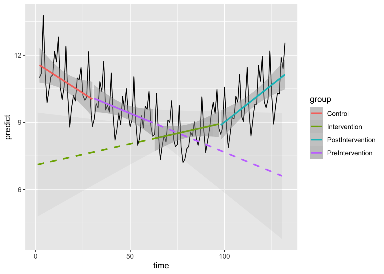
This is a neat trick, but in most circumstances you can probably make good use of an extrapolation from the truncated data as described in the section on Interrupted Time Series Analysis