Background
The sf package provides a seamless integration between R, ggplot, shapefiles, geoJSON and other GIS formats. A bonus here is that sf objects behave like dataframes so you can bind your own data on to an sf object and use your bound data to control things like putting chloropleths on the map.
This shamelessly copies a tutorial found here .
The rnaturalearth
Libraries
── Attaching core tidyverse packages ──────────────────────── tidyverse 2.0.0 ──
✔ dplyr     1.2.1     ✔ readr     2.2.0
✔ forcats   1.0.1     ✔ stringr   1.6.0
✔ ggplot2   4.0.3     ✔ tibble    3.3.1
✔ lubridate 1.9.5     ✔ tidyr     1.3.2
✔ purrr     1.2.2
── Conflicts ────────────────────────────────────────── tidyverse_conflicts() ──
✖ dplyr::filter() masks stats::filter()
✖ dplyr::lag()    masks stats::lag()
ℹ Use the conflicted package (<http://conflicted.r-lib.org/>) to force all conflicts to become errors
Linking to GEOS 3.14.1, GDAL 3.8.5, PROJ 9.5.1; sf_use_s2() is TRUE
library (knitr)library (ggspatial)library ("rnaturalearth" )library ("rnaturalearthdata" )
Attaching package: 'rnaturalearthdata'

The following object is masked from 'package:rnaturalearth':

    countries110
Data
#call the polygons <- ne_countries (scale = "medium" , returnclass = "sf" )
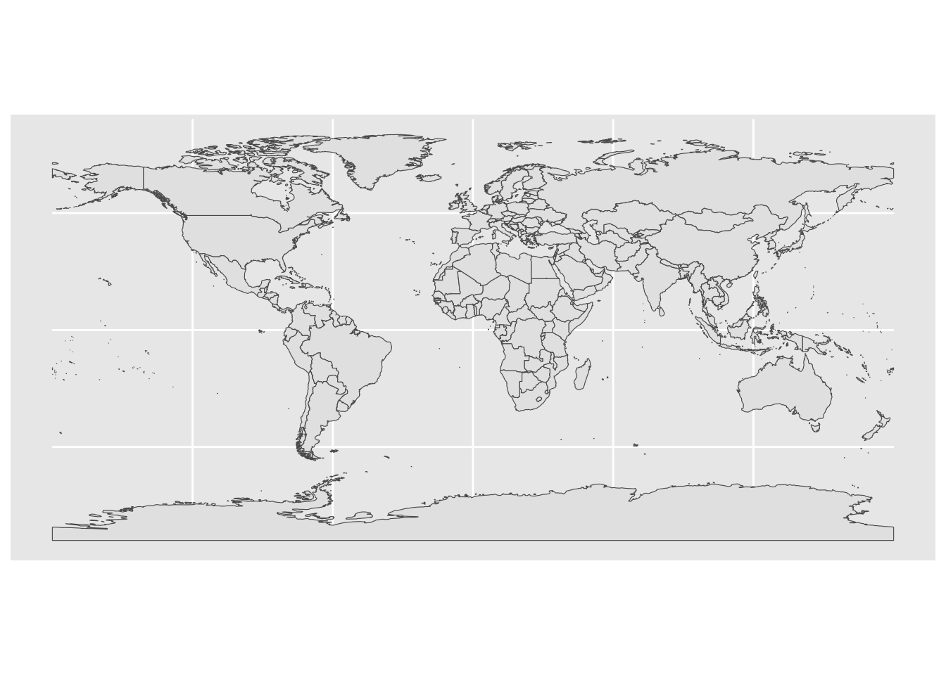
Draw basic polygons
ggplot (data = world) + geom_sf ()
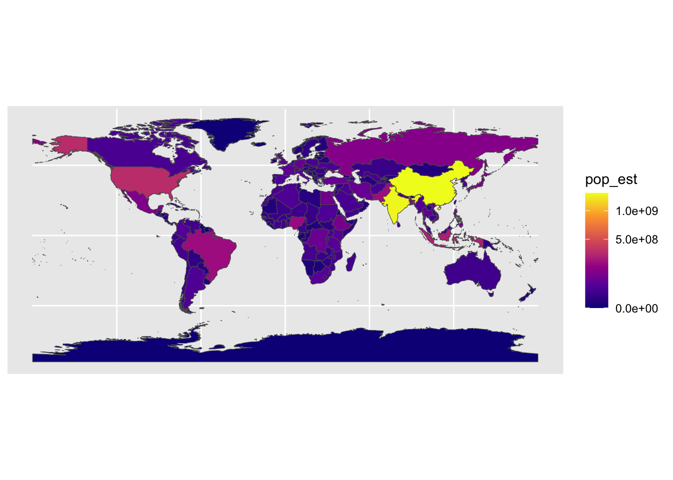
Colour the map with continuous variable
ggplot (data = world) + geom_sf (aes (fill = pop_est)) + scale_fill_viridis_c (option = "plasma" , trans = "sqrt" )
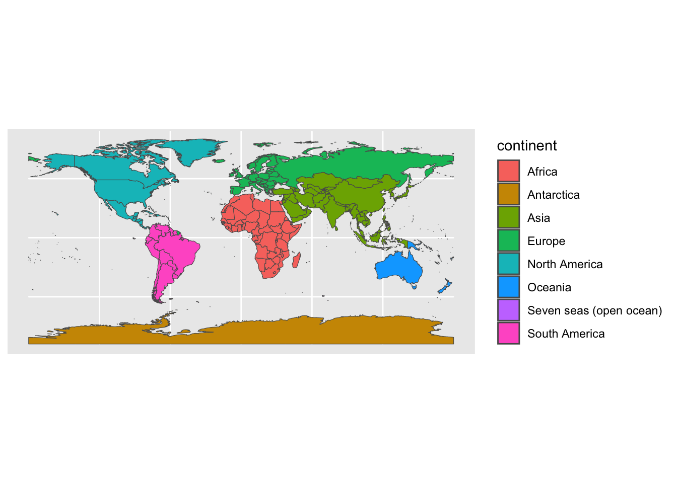
Colour the map with factor variable
ggplot (data = world) + geom_sf (aes (fill = continent))
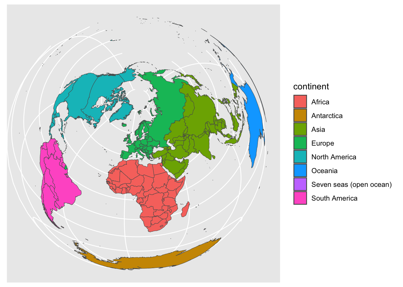
Change the projection with coord_sf
ggplot (data = world) + geom_sf (aes (fill = continent))+ coord_sf (crs = st_crs (3035 ))
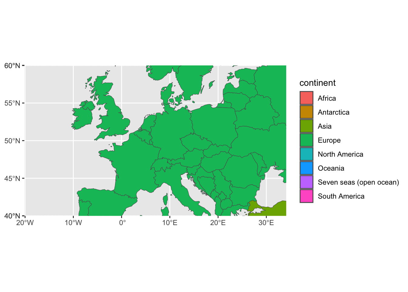
Focus on a specific region
ggplot (data = world) + geom_sf (aes (fill = continent))+ coord_sf (xlim = c (- 20.15 , 34.12 ), ylim = c (40 , 60 ), expand = FALSE )
Decorate with scale bar / compass
ggplot (data = world) + geom_sf (aes (fill = continent))+ coord_sf (xlim = c (- 20.15 , 34.12 ), ylim = c (40 , 60 ), expand = FALSE ) + annotation_scale (location = "br" , width_hint = 0.4 ) + annotation_north_arrow (location = "bl" , which_north = "true" , pad_x = unit (0.1 , "cm" ), pad_y = unit (0.3 , "cm" ),style = north_arrow_fancy_orienteering)
Scale on map varies by more than 10%, scale bar may be inaccurate
Identify centroids of each polygon
This will be used to place country name labels
= st_make_valid (world)<- st_centroid (world)
Warning: st_centroid assumes attributes are constant over geometries
<- cbind (world, st_coordinates (st_centroid (world$ geometry)))
Add labels
ggplot (data = world) + geom_sf (aes (fill = continent))+ coord_sf (xlim = c (- 20.15 , 34.12 ), ylim = c (40 , 60 ), expand = FALSE ) + annotation_scale (location = "br" , width_hint = 0.4 ) + annotation_north_arrow (location = "bl" , which_north = "true" , pad_x = unit (0.1 , "cm" ), pad_y = unit (0.3 , "cm" ),style = north_arrow_fancy_orienteering) + geom_text (data= world_points,aes (x= X, y= Y, label= name),color = "darkblue" , fontface = "bold" , check_overlap = FALSE ,size= 1.5
Scale on map varies by more than 10%, scale bar may be inaccurate
Add other pretty things
ggplot (data = world) + geom_sf (aes (fill = continent))+ coord_sf (xlim = c (- 20.15 , 34.12 ), ylim = c (40 , 60 ), expand = FALSE ) + annotation_scale (location = "br" , width_hint = 0.4 ) + annotation_north_arrow (location = "bl" , which_north = "true" , pad_x = unit (0.1 , "cm" ), pad_y = unit (0.3 , "cm" ),style = north_arrow_fancy_orienteering) + geom_text (data= world_points,aes (x= X, y= Y, label= name),color = "darkblue" , fontface = "bold" , check_overlap = FALSE ,size= 1.5 + theme (panel.grid.major = element_line (color = gray (.5 ), linetype = "dashed" , size = 0.5
Warning: The `size` argument of `element_line()` is deprecated as of ggplot2 3.4.0.
ℹ Please use the `linewidth` argument instead.
Scale on map varies by more than 10%, scale bar may be inaccurate
Save as PDF
ggsave (filename = "output/political_map.pdf" ,dpi = 300 )
Saving 7 x 5 in image
Scale on map varies by more than 10%, scale bar may be inaccurate
Test on new data from some shape files
Using shape files can be quite slow, so here we will only use a few polygons
download.file ("https://www.abs.gov.au/ausstats/subscriber.nsf/log?openagent&1270055004_sua_2016_aust_shape.zip&1270.0.55.004&Data%20Cubes&1E24D1FB300696D2CA2581B1000E15A5&0&July%202016&09.10.2017&Latest" ,destfile = "data/SUA_2016_AUST.zip" )unzip (zipfile = "data/SUA_2016_AUST.zip" ,exdir = "data/" )
Open Data
= read_sf ("data/SUA_2016_AUST.shp" ) = map [1 : 20 ,]
Plot map
ggplot (data = map) + geom_sf ()+ theme (panel.grid.major = element_line (color = gray (.5 ), linetype = "dashed" , size = 0.5 legend.position= "none"