library(tidyverse)
library(knitr)
library(data.table)
library(mclust)
library(mixtools)
install.packages("packages/lxb-1.5.tar.gz", repos = NULL, type="source")
library(lxb)21 Digital Luminex
21.0.1 Background
This script demonstrates how to read data from a Luminex .LXB file and to apply a ‘digital’ luminex approach. This counts the number of beads that fluoresce above a threshold, rather than looking at the mean fluorescence intensity for a marker on all beads. This is analogous to a ‘digital PCR’ approach.
In theory this might be a method that requires less inter-plate normalisation as the method is less dependent on average signal strength and more dependent on a within-plate EM model that simply asks what fraction of beads have a positive signal for each marker. Specifically, the actual fluorescence intensity of the markers on the beads is actually very variable from plate to plate, but whatever the fluorescence intensity is, it should still be possible to define a positive and negative population.
The work uses an approach to reading the LXB files which was originally implemented in the lxb package. This is no longer maintained, so a copy of the tar file is included in the packages directory of this repo.
21.1 Libraries
21.2 Define Functions
21.2.1 Convert LXB Files to CSV
Create function to import an lxb file, add the well name, convert to a data frame and export a CSV with similar name to original file.
lxb.parse<-function(lxbfile)
{
#get the file
outputfile<-gsub(x = lxbfile,pattern = ".lxb",replacement = ".csv")
well<-unlist(strsplit(lxbfile,split = "_"))
well<-well[length(well)]
well<-gsub(well,pattern = ".lxb",replacement = "")
lxbdata <- readLxb(lxbfile)
lxbdata <- as.data.frame(lxbdata)
names(lxbdata)<-gsub(names(lxbdata),pattern = " ",replacement = ".")
lxbdata$well<-well
#remove invalid beads
lxbdata<-lxbdata[which(lxbdata$Bead.Valid==1),]
write.csv(x = lxbdata,file = outputfile,row.names = F)
}
21.2.2 Aggregate the csv files in a single df
#define a function to
lxb.aggregate.data<-function(path)
{
  #list only the csv files
  lxbs<-list.files(path = path,pattern = "*.csv",full.names = T)
  tables <- lapply(lxbs, fread)
  data.table::rbindlist(tables)
}
21.2.3 Apply mixed EM to find thresholds on each bead
lxb.digital.thresholds<-function(df,pdf.out=FALSE,sd.threshold=5)
{
  df2<-df %>% group_by(Bead.ID) %>% summarise(n=n())
  #get bead values from DF
  df2$EM.threshold<-NA

  for(i in 1:length(df2$Bead.ID))
  {
    fit<-normalmixEM(df$RP1L.Peak[which(df$Bead.ID==df2$Bead.ID[i])])
    #plot(fit,which=2,breaks=40)

    df2$EM.threshold[i]<-fit$mu[which(fit$mu==min(fit$mu))]+(sd.threshold*fit$sigma[which(fit$mu==min(fit$mu))])
    if(pdf.out==TRUE){
                      pdf(file = paste("data/Luminex_LXB_Files/",df2$Bead.ID[i],".pdf",sep=""))
                      par(mfrow=c(1,2))
                      plot(sort(df$RP1L.Peak[which(df$Bead.ID==df2$Bead.ID[i])]))
                      abline(h=df2$EM.threshold[i],lty=2,col="red")
                      plot(fit,whichplots = 2)
                      abline(v=df2$EM.threshold[i],lty=2,col="red")
                                        dev.off()
                      }
  }
  df<-merge(df,df2,by="Bead.ID")
  print(df2)
  df$classification<-as.numeric(df$RP1L.Peak>df$EM.threshold)
  return(df)
}
21.2.4 Manually select threshold values
lxb.digital.thresholds.locator<-function(df,pdf.out=FALSE,sd.threshold=4)
{
  df2<-df %>% group_by(Bead.ID) %>% summarise(n=n())
  #get bead values from DF
  df2$EM.threshold<-NA
  df2$EM.threshold<-as.numeric(df2$EM.threshold)

  for(i in 1:length(df2$Bead.ID))
  {
    fit<-normalmixEM(df$RP1L.Peak[which(df$Bead.ID==df2$Bead.ID[i])])
    #plot(fit,which=2,breaks=40)


      plot(fit,whichplots = 2)
      EM.threshold<-locator(n = 1)
      df2$EM.threshold[i]<-EM.threshold$x
      abline(v=df2$EM.threshold[i],lty=2,col="red")
  }


  df<-merge(df,df2,by="Bead.ID")
  print(df2)
  df$classification<-as.numeric(df$RP1L.Peak>df$EM.threshold)
  return(df)
}
21.3 Apply the functions to real data
21.3.1 List the LXB files
Luminex machines spit out one LXB file for each well
lxbs<-list.files(path = "data/Luminex_LXB_Files/",pattern = "*.lxb",full.names = T)
lxbs
[1] "data/Luminex_LXB_Files//A1.lxb" "data/Luminex_LXB_Files//A10.lxb"
[3] "data/Luminex_LXB_Files//A11.lxb" "data/Luminex_LXB_Files//A12.lxb"
[5] "data/Luminex_LXB_Files//A2.lxb" "data/Luminex_LXB_Files//A3.lxb"
[7] "data/Luminex_LXB_Files//A4.lxb" "data/Luminex_LXB_Files//A5.lxb"
[9] "data/Luminex_LXB_Files//A6.lxb" "data/Luminex_LXB_Files//A7.lxb"
[11] "data/Luminex_LXB_Files//A8.lxb" "data/Luminex_LXB_Files//A9.lxb" 21.3.2 Apply the lxb.parse function to all lxb files in directory
lapply(lxbs,lxb.parse)[[1]]
NULL
[[2]]
NULL
[[3]]
NULL
[[4]]
NULL
[[5]]
NULL
[[6]]
NULL
[[7]]
NULL
[[8]]
NULL
[[9]]
NULL
[[10]]
NULL
[[11]]
NULL
[[12]]
NULL21.3.3 Aggregate the data
a<-lxb.aggregate.data(path = "data/Luminex_LXB_Files/")
a$col<-substr(a$well,start = 1,stop = 1)
a$row<-substr(a$well,start = 2,stop = 3)
kable(head(a,20))| CL1.X | CL1.Y | CL1.Peak | CL1.Ch.Value | CL1.Area | CL1.Valid | CL1.SR | CL1.MBR | CL1.Pass.Mini.Ratio | CL1.Pass.Max.Ratio | CL1.Pass.Nearby | CL1.Pass.Edge | CL2.X | CL2.Y | CL2.Peak | CL2.Ch.Value | CL2.Area | CL2.Valid | CL2.SR | CL2.MBR | CL2.Pass.Mini.Ratio | CL2.Pass.Max.Ratio | CL2.Pass.Nearby | CL2.Pass.Edge | RP1L.X | RP1L.Y | RP1L.Peak | RP1L.Ch.Value | RP1L.Area | RP1L.Valid | RP1L.SR | RP1L.MBR | RP1L.Pass.Mini.Ratio | RP1L.Pass.Max.Ratio | RP1L.Pass.Nearby | RP1L.Pass.Edge | RP1S.X | RP1S.Y | RP1S.Peak | RP1S.Ch.Value | RP1S.Area | RP1S.Valid | RP1S.SR | RP1S.MBR | RP1S.Pass.Mini.Ratio | RP1S.Pass.Max.Ratio | RP1S.Pass.Nearby | RP1S.Pass.Edge | Bead.Valid | CL2.Offset.X | CL2.Offset.Y | CL1_CL2.Dist | RP1.Offset.X | RP1.Offset.Y | CL1.Value | CL2.Value | RP1.Value | Bead.ID | well | col | row |
|---|---|---|---|---|---|---|---|---|---|---|---|---|---|---|---|---|---|---|---|---|---|---|---|---|---|---|---|---|---|---|---|---|---|---|---|---|---|---|---|---|---|---|---|---|---|---|---|---|---|---|---|---|---|---|---|---|---|---|---|---|
| 1149234516 | 1092558165 | 1343 | 0 | 16947 | 1 | -1560336802 | -462012473 | 1 | 1 | 1 | 1 | 1149223297 | 1092479444 | 1296 | 0 | 16974 | 1 | 1181464885 | -1991868891 | 1 | 1 | 1 | 1 | 1149236985 | 1092988697 | 59632 | 0 | 1135332 | 1 | 0 | 0 | 1 | 1 | 1 | 1 | 1149236985 | 1092988697 | 59632 | 0 | 52185 | 1 | 0 | 0 | 1 | 1 | 1 | 1 | 1 | 0 | 0 | -812668335 | 0 | 0 | 118 | 118 | 6103 | 12 | Files//A1 | F | il |
| 1155884337 | 1093973789 | 2535 | 0 | 32248 | 1 | -1461695296 | -1174163721 | 1 | 1 | 1 | 1 | 1155877959 | 1094254143 | 3861 | 0 | 49562 | 1 | 1419346258 | -463449520 | 1 | 1 | 1 | 1 | 1155884214 | 1094404032 | 49395 | 0 | 777699 | 1 | 0 | 0 | 1 | 1 | 1 | 1 | 1155884214 | 1094404032 | 49395 | 0 | 27587 | 1 | 0 | 0 | 1 | 1 | 1 | 1 | 1 | 0 | 0 | -1717978224 | 0 | 0 | 224 | 345 | 3080 | 26 | Files//A1 | F | il |
| 1141831731 | 1094397512 | 7971 | 0 | 100698 | 1 | 681421247 | -1790273464 | 1 | 1 | 1 | 1 | 1141820439 | 1093943886 | 2157 | 0 | 26850 | 1 | -402982476 | -53427154 | 1 | 1 | 1 | 1 | 1141835711 | 1094827668 | 61485 | 0 | 1217522 | 1 | 0 | 0 | 1 | 1 | 1 | 1 | 1141835711 | 1094827668 | 61485 | 0 | 63810 | 1 | 0 | 0 | 1 | 1 | 1 | 1 | 1 | 0 | 0 | 1367863707 | 0 | 0 | 701 | 187 | 7463 | 21 | Files//A1 | F | il |
| 1150917202 | 1097198649 | 4966 | 0 | 60897 | 1 | 271482799 | -1191083431 | 1 | 1 | 1 | 1 | 1150911874 | 1097454201 | 4016 | 0 | 50462 | 1 | 1850697676 | -113029935 | 1 | 1 | 1 | 1 | 1150918093 | 1097628233 | 61767 | 0 | 1249945 | 1 | 0 | 0 | 1 | 1 | 1 | 1 | 1150918093 | 1097628233 | 61767 | 0 | 80109 | 1 | 0 | 0 | 1 | 1 | 1 | 1 | 1 | 0 | 0 | 459537696 | 0 | 0 | 424 | 352 | 9369 | 27 | Files//A1 | F | il |
| 1152361617 | 1097643907 | 16662 | 0 | 208370 | 1 | -351809365 | -2047823587 | 1 | 1 | 1 | 1 | 1152359059 | 1097576007 | 2136 | 0 | 28456 | 1 | 2107587046 | 76070548 | 1 | 1 | 1 | 1 | 1152362214 | 1098073401 | 59204 | 0 | 848208 | 1 | 0 | 0 | 1 | 1 | 1 | 1 | 1152362214 | 1098073401 | 59204 | 0 | 33077 | 1 | 0 | 0 | 1 | 1 | 1 | 1 | 1 | 0 | 0 | -1127313627 | 0 | 0 | 1450 | 198 | 3868 | 22 | Files//A1 | F | il |
| 1151775855 | 1098727795 | 16030 | 0 | 203329 | 1 | 870860878 | 1513437910 | 1 | 1 | 1 | 1 | 1151770676 | 1098681510 | 3822 | 0 | 47775 | 1 | -758130026 | 1252485282 | 1 | 1 | 1 | 1 | 1151776571 | 1099032358 | 14198 | 0 | 166583 | 1 | 0 | 0 | 1 | 1 | 1 | 1 | 1151776571 | 1099032358 | 14198 | 0 | 5589 | 1 | 0 | 0 | 1 | 1 | 1 | 1 | 1 | 0 | 0 | 1774791597 | 0 | 0 | 1415 | 333 | 660 | 29 | Files//A1 | F | il |
| 1155033097 | 1100340701 | 4580 | 0 | 59419 | 1 | -1852063166 | -1009139138 | 1 | 1 | 1 | 1 | 1155030331 | 1100114914 | 3966 | 0 | 51219 | 1 | 114335912 | -500949543 | 1 | 1 | 1 | 1 | 1155033148 | 1100555026 | 61894 | 0 | 1325814 | 1 | 0 | 0 | 1 | 1 | 1 | 1 | 1155033148 | 1100555026 | 61894 | 0 | 81886 | 1 | 0 | 0 | 1 | 1 | 1 | 1 | 1 | 0 | 0 | -730158204 | 0 | 0 | 414 | 357 | 9577 | 27 | Files//A1 | F | il |
| 1156429977 | 1102179833 | 15608 | 0 | 198756 | 1 | 1505756983 | 1583439109 | 1 | 1 | 1 | 1 | 1156424231 | 1102098349 | 2208 | 0 | 28248 | 1 | -1090034562 | 391667932 | 1 | 1 | 1 | 1 | 1156429743 | 1102393783 | 59594 | 0 | 1228318 | 1 | 0 | 0 | 1 | 1 | 1 | 1 | 1156429743 | 1102393783 | 59594 | 0 | 53059 | 1 | 0 | 0 | 1 | 1 | 1 | 1 | 1 | 0 | 0 | 493372241 | 0 | 0 | 1383 | 197 | 6205 | 22 | Files//A1 | F | il |
| 1133053433 | 1102435101 | 2559 | 0 | 32062 | 1 | -1841237300 | -413394956 | 1 | 1 | 1 | 1 | 1133042566 | 1102219953 | 1325 | 0 | 16486 | 1 | 926199853 | 962368627 | 1 | 1 | 1 | 1 | 1133063386 | 1102648999 | 40484 | 0 | 566360 | 1 | 0 | 0 | 1 | 1 | 1 | 1 | 1133063386 | 1102648999 | 40484 | 0 | 20078 | 1 | 0 | 0 | 1 | 1 | 1 | 1 | 1 | 0 | 0 | 2138917700 | 0 | 0 | 223 | 115 | 2243 | 13 | Files//A1 | F | il |
| 1146917648 | 1102574438 | 15451 | 0 | 199489 | 1 | 9330036 | -2058791451 | 1 | 1 | 1 | 1 | 1146911794 | 1102523540 | 2114 | 0 | 26610 | 1 | 1844585360 | -208857109 | 1 | 1 | 1 | 1 | 1146920590 | 1102788307 | 59663 | 0 | 1092730 | 1 | 0 | 0 | 1 | 1 | 1 | 1 | 1146920590 | 1102788307 | 59663 | 0 | 45526 | 1 | 0 | 0 | 1 | 1 | 1 | 1 | 1 | 0 | 0 | -1874985181 | 0 | 0 | 1388 | 185 | 5324 | 22 | Files//A1 | F | il |
| 1132034886 | 1104184846 | 15495 | 0 | 196309 | 1 | -614810869 | -1382596637 | 1 | 1 | 1 | 1 | 1132011269 | 1104132015 | 2002 | 0 | 27293 | 1 | -1153969394 | -422053358 | 1 | 1 | 1 | 1 | 1132055122 | 1104398386 | 60985 | 0 | 1203448 | 1 | 0 | 0 | 1 | 1 | 1 | 1 | 1132055122 | 1104398386 | 60985 | 0 | 51501 | 1 | 0 | 0 | 1 | 1 | 1 | 1 | 1 | 0 | 0 | -199422534 | 0 | 0 | 1366 | 190 | 6023 | 22 | Files//A1 | F | il |
| 1148738278 | 1104800157 | 2225 | 0 | 30448 | 1 | 336334840 | -1722049420 | 1 | 1 | 1 | 1 | 1148727247 | 1104737582 | 2088 | 0 | 27703 | 1 | -1264850604 | 711461030 | 1 | 1 | 1 | 1 | 1148740848 | 1105013572 | 4811 | 0 | 52665 | 1 | 0 | 0 | 1 | 1 | 1 | 1 | 1148740848 | 1105013572 | 4811 | 0 | 1513 | 1 | 0 | 0 | 1 | 1 | 1 | 1 | 1 | 0 | 0 | 1664716139 | 0 | 0 | 212 | 193 | 209 | 19 | Files//A1 | F | il |
| 1154128511 | 1104521200 | 16433 | 0 | 201733 | 1 | -1224775220 | -434514866 | 1 | 1 | 1 | 1 | 1154122887 | 1104494251 | 3611 | 0 | 47364 | 1 | 317673209 | 429097738 | 1 | 1 | 1 | 1 | 1154128747 | 1104734672 | 14749 | 0 | 226132 | 1 | 0 | 0 | 1 | 1 | 1 | 1 | 1154128747 | 1104734672 | 14749 | 0 | 7379 | 1 | 0 | 0 | 1 | 1 | 1 | 1 | 1 | 0 | 0 | -510452285 | 0 | 0 | 1404 | 330 | 895 | 29 | Files//A1 | F | il |
| 1121352736 | 1105125885 | 4568 | 0 | 58170 | 1 | 1999822347 | 898421215 | 1 | 1 | 1 | 1 | 1121307392 | 1105088368 | 1294 | 0 | 16234 | 1 | -983333522 | -1739258039 | 1 | 1 | 1 | 1 | 1121397014 | 1105339233 | 6723 | 0 | 93542 | 1 | 0 | 0 | 1 | 1 | 1 | 1 | 1121397014 | 1105339233 | 6723 | 0 | 2880 | 1 | 0 | 0 | 1 | 1 | 1 | 1 | 1 | 0 | 0 | 1329047872 | 0 | 0 | 405 | 113 | 370 | 14 | Files//A1 | F | il |
| 1155909558 | 1106777421 | 1199 | 0 | 16460 | 1 | 821266378 | -1246218943 | 1 | 1 | 1 | 1 | 1155906397 | 1106722413 | 2283 | 0 | 29468 | 1 | 1183943161 | -426756626 | 1 | 1 | 1 | 1 | 1155909430 | 1106990432 | 17653 | 0 | 332506 | 1 | 0 | 0 | 1 | 1 | 1 | 1 | 1155909430 | 1106990432 | 17653 | 0 | 11300 | 1 | 0 | 0 | 1 | 1 | 1 | 1 | 1 | 0 | 0 | -250784161 | 0 | 0 | 115 | 205 | 1317 | 18 | Files//A1 | F | il |
| 1155824328 | 1107578705 | 4538 | 0 | 59342 | 1 | 1559411272 | 1151799898 | 1 | 1 | 1 | 1 | 1155818790 | 1107546496 | 4086 | 0 | 51988 | 1 | -919791236 | 351277236 | 1 | 1 | 1 | 1 | 1155824218 | 1107685100 | 60610 | 0 | 1258483 | 1 | 0 | 0 | 1 | 1 | 1 | 1 | 1155824218 | 1107685100 | 60610 | 0 | 58400 | 1 | 0 | 0 | 1 | 1 | 1 | 1 | 1 | 0 | 0 | 1128053269 | 0 | 0 | 413 | 362 | 6830 | 27 | Files//A1 | F | il |
| 1155536851 | 1108324761 | 15984 | 0 | 204814 | 1 | 27751286 | 468010390 | 1 | 1 | 1 | 1 | 1155531489 | 1108306151 | 3837 | 0 | 49674 | 1 | -124177506 | 392542407 | 1 | 1 | 1 | 1 | 1155536799 | 1108431004 | 27421 | 0 | 513624 | 1 | 0 | 0 | 1 | 1 | 1 | 1 | 1155536799 | 1108431004 | 27421 | 0 | 17913 | 1 | 0 | 0 | 1 | 1 | 1 | 1 | 1 | 0 | 0 | 583326885 | 0 | 0 | 1426 | 346 | 2034 | 29 | Files//A1 | F | il |
| 1155406742 | 1108697607 | 2641 | 0 | 33191 | 1 | -1232077645 | -149200003 | 1 | 1 | 1 | 1 | 1155400871 | 1108654290 | 2163 | 0 | 29448 | 1 | 0 | 2050056381 | 1 | 1 | 1 | 1 | 1155406717 | 1108803773 | 3061 | 0 | 42222 | 1 | 0 | 0 | 1 | 1 | 1 | 1 | 1155406717 | 1108803773 | 3061 | 0 | 1392 | 1 | 0 | 0 | 1 | 1 | 1 | 1 | 1 | 0 | 0 | -1202766431 | 0 | 0 | 231 | 205 | 167 | 19 | Files//A1 | F | il |
| 1156984613 | 1108597201 | 1279 | 0 | 16629 | 1 | -1691806559 | -659651601 | 1 | 1 | 1 | 1 | 1156981428 | 1108475694 | 2288 | 0 | 29547 | 1 | -763044262 | 583186408 | 1 | 1 | 1 | 1 | 1156984266 | 1108703388 | 47656 | 0 | 1013692 | 1 | 0 | 0 | 1 | 1 | 1 | 1 | 1156984266 | 1108703388 | 47656 | 0 | 36156 | 1 | 0 | 0 | 1 | 1 | 1 | 1 | 1 | 0 | 0 | -1178951951 | 0 | 0 | 116 | 206 | 4014 | 18 | Files//A1 | F | il |
| 1142762190 | 1109171906 | 4698 | 0 | 58567 | 1 | 1518863941 | -1049339851 | 1 | 1 | 1 | 1 | 1142752128 | 1109138271 | 2183 | 0 | 28897 | 1 | 1038826580 | -1612340562 | 1 | 1 | 1 | 1 | 1142765981 | 1109277976 | 39473 | 0 | 517176 | 1 | 0 | 0 | 1 | 1 | 1 | 1 | 1142765981 | 1109277976 | 39473 | 0 | 18003 | 1 | 0 | 0 | 1 | 1 | 1 | 1 | 1 | 0 | 0 | -1169600992 | 0 | 0 | 408 | 201 | 2048 | 20 | Files//A1 | F | il |
21.3.4 Trim data to beads we actually used
The data may include beads that weren’t used in the assay. Here we used a subset of beads and so need to filter the data
a<-subset(a, subset = Bead.ID %in% c(12:15,18,19,20,21,22,25:30))21.3.5 Plot data for all beads
CL1 and CL2 are the bead identification lasers.
ggplot(data = a,aes(x=CL1.Peak,y=CL2.Peak,color=factor(Bead.ID)))+geom_point()+
  scale_x_continuous(trans = "log")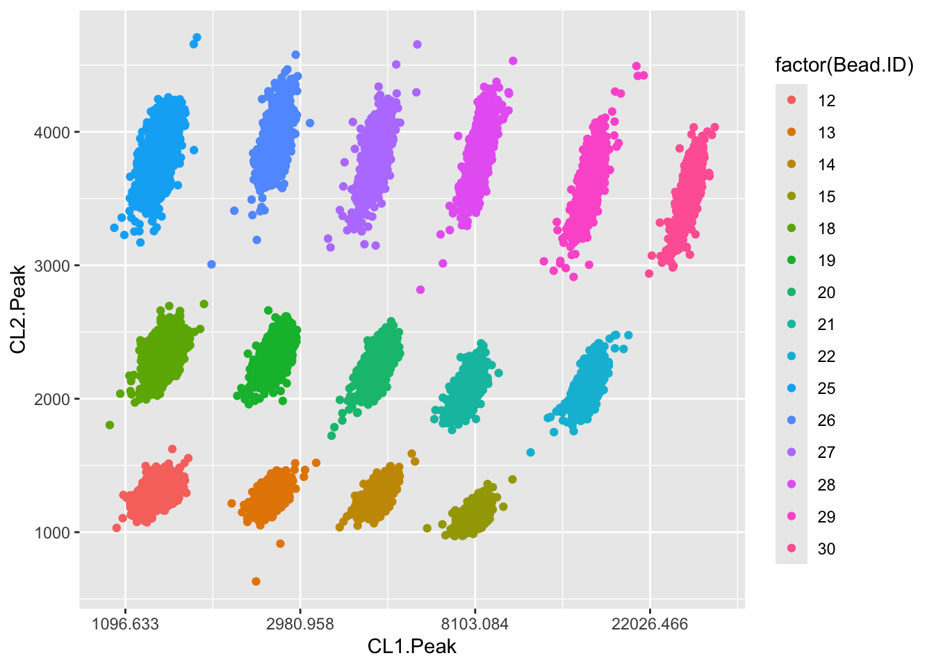
21.3.6 Show table of bead counts
table(factor(a$Bead.ID),a$Bead.Valid)
        1
  12 1554
  13 1183
  14 1482
  15 1283
  18 1711
  19 1607
  20 1375
  21 1536
  22 1567
  25 1684
  26 1347
  27 1775
  28 1490
  29 1634
  30 1150
21.3.7 Threshold classify everything based on automated EM algorithm
This also saves a PDF in the directory data/Luminex_LXB_Files/
a<-lxb.digital.thresholds(a,pdf.out = T,sd.threshold = 3)number of iterations= 13 number of iterations= 58 number of iterations= 43 number of iterations= 28 number of iterations= 74 number of iterations= 44 number of iterations= 21 number of iterations= 26 number of iterations= 47 number of iterations= 48 number of iterations= 36 number of iterations= 24 number of iterations= 262 number of iterations= 92 number of iterations= 20 # A tibble: 15 × 3
Bead.ID n EM.threshold
<int> <int> <dbl>
1 12 1554 82664.
2 13 1183 27482.
3 14 1482 18306.
4 15 1283 13884.
5 18 1711 49013.
6 19 1607 11781.
7 20 1375 8491.
8 21 1536 10624.
9 22 1567 22790.
10 25 1684 21194.
11 26 1347 14887.
12 27 1775 95263.
13 28 1490 8797.
14 29 1634 12463.
15 30 1150 90940.21.4 Summarise based on bead counts
aa<-a %>% group_by(Bead.ID,well) %>% summarise(count=n(),bead.pos=sum(classification==1),bead.neg=sum(classification==0),bead.fraction=(bead.pos=sum(classification==1)/n()))
aa$col<-substr(aa$well,start = 1,stop = 1)
aa$row<-substr(aa$well,start = 2,stop = 3)


kable(head(aa,24))| Bead.ID | well | count | bead.pos | bead.neg | bead.fraction | col | row |
|---|---|---|---|---|---|---|---|
| 12 | Files//A1 | 70 | 0 | 70 | 0.0000000 | F | il |
| 12 | Files//A10 | 161 | 0 | 161 | 0.0000000 | F | il |
| 12 | Files//A11 | 139 | 0 | 139 | 0.0000000 | F | il |
| 12 | Files//A12 | 134 | 0 | 134 | 0.0000000 | F | il |
| 12 | Files//A2 | 119 | 0 | 119 | 0.0000000 | F | il |
| 12 | Files//A3 | 139 | 0 | 139 | 0.0000000 | F | il |
| 12 | Files//A4 | 119 | 0 | 119 | 0.0000000 | F | il |
| 12 | Files//A5 | 135 | 0 | 135 | 0.0000000 | F | il |
| 12 | Files//A6 | 151 | 0 | 151 | 0.0000000 | F | il |
| 12 | Files//A7 | 117 | 0 | 117 | 0.0000000 | F | il |
| 12 | Files//A8 | 141 | 0 | 141 | 0.0000000 | F | il |
| 12 | Files//A9 | 129 | 0 | 129 | 0.0000000 | F | il |
| 13 | Files//A1 | 57 | 25 | 32 | 0.4385965 | F | il |
| 13 | Files//A10 | 119 | 0 | 119 | 0.0000000 | F | il |
| 13 | Files//A11 | 88 | 4 | 84 | 0.0454545 | F | il |
| 13 | Files//A12 | 114 | 3 | 111 | 0.0263158 | F | il |
| 13 | Files//A2 | 102 | 35 | 67 | 0.3431373 | F | il |
| 13 | Files//A3 | 106 | 3 | 103 | 0.0283019 | F | il |
| 13 | Files//A4 | 88 | 6 | 82 | 0.0681818 | F | il |
| 13 | Files//A5 | 87 | 4 | 83 | 0.0459770 | F | il |
| 13 | Files//A6 | 107 | 8 | 99 | 0.0747664 | F | il |
| 13 | Files//A7 | 88 | 4 | 84 | 0.0454545 | F | il |
| 13 | Files//A8 | 114 | 76 | 38 | 0.6666667 | F | il |
| 13 | Files//A9 | 113 | 5 | 108 | 0.0442478 | F | il |
21.5 Interpretation
The bead.fraction is the fraction of all beads in the well which were above the n SD threshold for positivity. This is a digital count converted in to a fraction, which allows a continuous measure to be gained for each
ggplot(aa,aes(well,bead.fraction))+
  geom_bar(stat="identity")+
  facet_wrap(.~Bead.ID)+
  theme(axis.text.x = element_text(angle = 90, vjust = 0.5, hjust=1))