This protocol can be used to confirm that antibodies have been correctly conjugated to beads. It works by using anti-species antibodies. Anti mouse-biotin is diluted in a series and reacted with the newly coupled beads which are coupled to mouse and rat antibodies.
On first use of the anti mouse-biotin, rehydrate it to be 0.2 mg/mL and aliquot into small volumes for freezer storage to minimise freeze-thaw cycles.
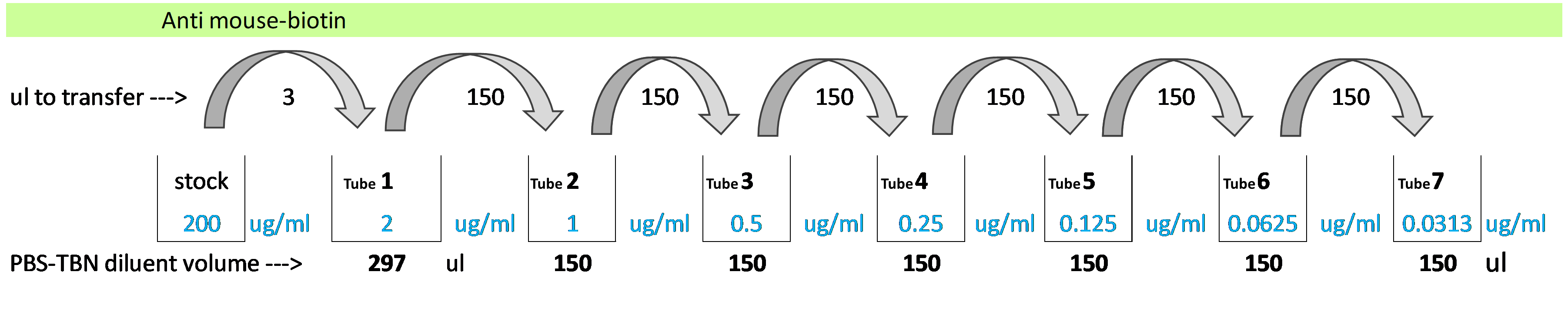
Thaw an aliquot of anti mouse-biotin, 3 µL is required for running two columns on a plate.
Add 900 µL of PBS-TBN to a tube for diluting the beads.
Get the newly coupled beads, vortex then sonicate for 20 s of each.
Add 2.4 µL of each newly-coupled bead to the 900 µL and vortex mix. (To give a theoretical 20,000 beads/mL, or 1000 beads/well, assuming 7.5x10⁶ beads/mL stock).
Label 7 tubes (1-7) for the anti mouse-biotin dilutions, corresponding to concentrations: 2, 1, 0.5, 0.25, 0.125, 0.063, 0.031 µg/mL.
Dispense PBS-TBN diluent into each tube in the volumes indicated in the bottom row of Figure 1.
Serially dilute anti mouse-biotin in PBS-TBN by adding 3 µL of the 0.2 mg/mL stock into Tube 1 (297 µL PBS-TBN) and transferring 150 µL of this into 150 µL PBS-TBN sequentially until Tube 7, vortex mixing between pipetting (Figure 1).
Figure 1. Dilution series of anti mouse biotin.
Dispense 50 µL/well of the diluted beads into two columns of a black plate as per plate layout below.
Wash beads once: Put plate on magnet, wait 60 s, invert plate on magnet to empty the liquid. Add 100 µL/well PBST, removing from the magnet when adding wash buffer. Replace plate on magnet for 60 s and remove liquid as before, dabbing gently on tissue before adding the next reagent.
Add 50 µL/well of the anti mouse-biotin dilutions (1-7) in duplicate, and 50 µL PBS-TBN as the blank, as per plate layout:
1
2
A
2.00 µg/mL
2.00 µg/mL
B
1.00 µg/mL
1.00 µg/mL
C
0.50 µg/mL
0.50 µg/mL
D
0.25 µg/mL
0.25 µg/mL
E
0.125 µg/mL
0.125 µg/mL
F
0.063 µg/mL
0.063 µg/mL
G
0.031 µg/mL
0.031 µg/mL
H
Blank 0 µg/mL
Blank 0 µg/mL
Cover and incubate on shaker for 45 mins at ambient temperature.
During the incubation, dilute SA-PE to 3 µg/mL by adding 2.7 µL of SA-PE to 900 µL PBS-TBN. Store this in the fridge until use.
Wash plate 3 times as before with 100 uL/well PBST.
Add 50 µL/well of diluted SA-PE to the plate.
Cover & incubate on shaker for 45 mins.
Wash plate 3 times as before with 100 µL/well PBST.
Add 100 µL PBS-TBN to each well and read on MagPix the same day using the 12-plex protocol.
For this analysis, we use only the median fluorescence data and only need to include the rows of the mfi data which relate to the experiments where a biotinylated, anti-mouse antibody was directed against the assay specific, antibody-coupled microbeads.
The basic steps include
Loading the csv file, renaming problematic columns
Removing headers from the MagPix output file
Filtering the data to include only MFI data
Filtering the MFI data to include only the relevant lines of data
Pivoting the data in to a tidy format
Charting the data
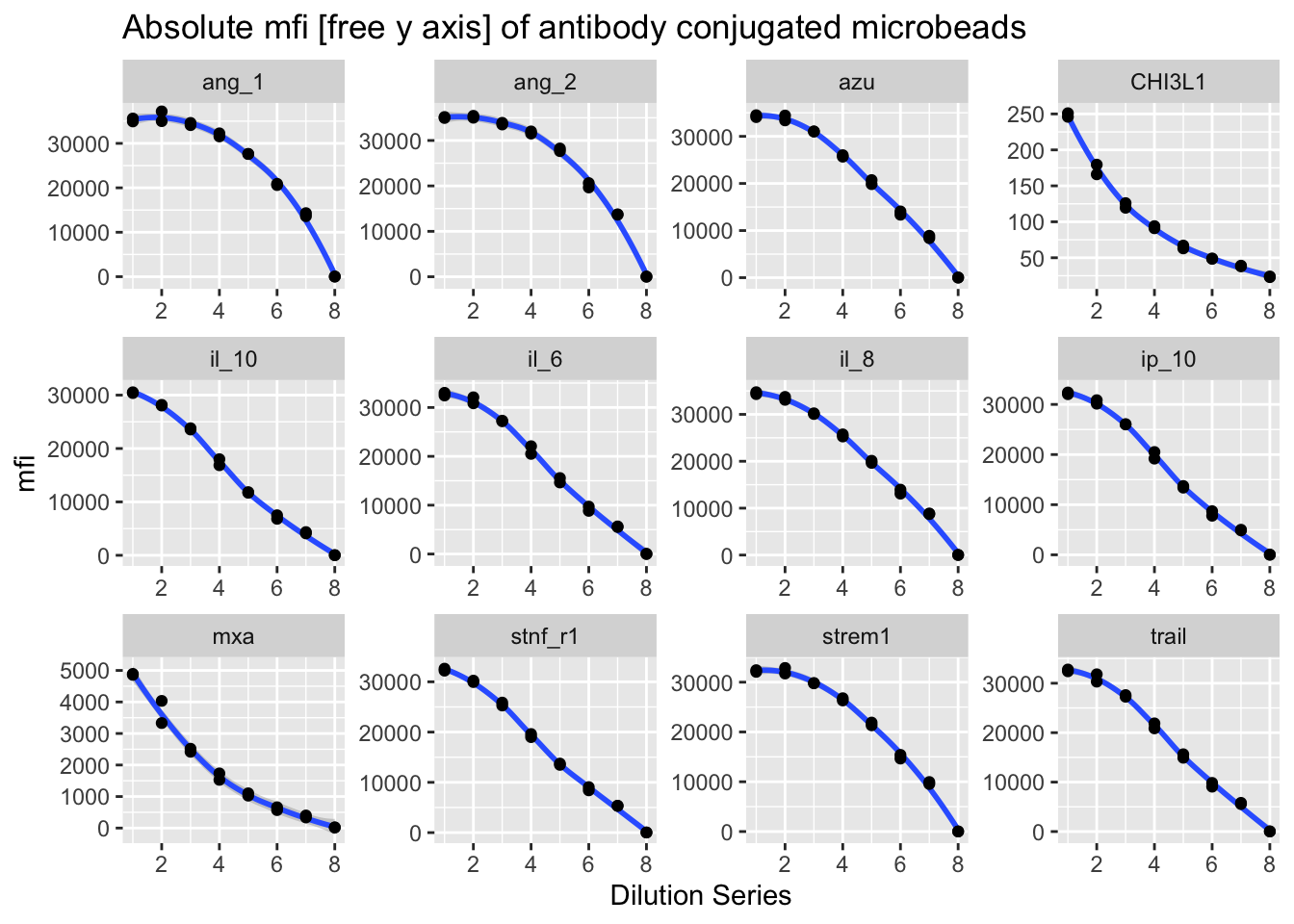
library(tidyverse)# read data in to dfdf<-suppressMessages(read_csv("data/coupling_confirmation/Bead_Coupling_Data.csv",skip =41,na =c("","NA","NaN"),show_col_types = F))%>%setNames(tolower(gsub("-","_",names(.)))) %>%mutate(sample=fct_explicit_na(sample)) %>%select_if(!names(.) %in%c('...16','...17', 'location', 'total events')) %>%rename_at(vars(matches("^CH3L1$")), function(x) "CHI3L1")#remove extraneous lines and keep only mfi data for anti-mouse biotinylated detection antibodies.df <- df[49:64,]#pivot datadf <- df %>%pivot_longer(cols=(-sample),names_to ="marker",values_to ="mfi") %>%separate(col = sample,into =c("sample","dilution"),sep ="biotin ") %>%mutate(dilution =as.numeric(dilution))ggplot(df,aes(as.numeric(dilution),as.numeric(mfi)))+geom_smooth(method ='loess',formula ='y ~ x')+geom_point()+facet_wrap(.~marker,scales ="free")+xlab("Dilution Series")+ylab("mfi")+ggtitle("Absolute mfi [free y axis] of antibody conjugated microbeads")
The chart above confirms that these microbeads (a) have successfully coupled to the assay specific mouse and rat antibodies and (b) that the MFI response varies in response to serial dilution of the biotinylated anti-mouse secondary antibody.
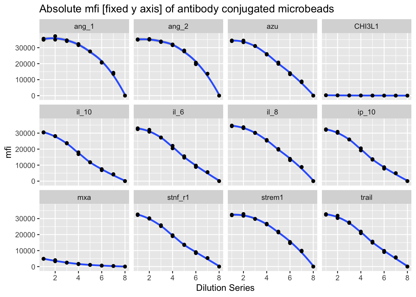
ggplot(df,aes(as.numeric(dilution),as.numeric(mfi)))+geom_smooth(method ="loess",formula ="y~x")+geom_point()+facet_wrap(.~marker,scales ="fixed")+xlab("Dilution Series")+ylab("mfi")+ggtitle("Absolute mfi [fixed y axis] of antibody conjugated microbeads")
When charted on a fixed y axis, it becomes clearer that some markers (i.e. CHI3L1 and MxA) have a much lower MFI across the full range of dilutions. This could be explained by lower avidity or affinity between the primary and secondary antibodies. This is likely the case for the CHI3L1 antibody which is from rat and exhibits low reactivity with the anti mouse-biotin. Low signal could also indicate steric effects, or experimental issues and failure to couple efficiently which may indicate that the beads are not useable.
Note that whilst both MxA and CHI3L1 both had lower MFI values than other markers, they still exhibited a dose-response curve that seems appropriate for experimental use. Assays such as MxA and CHI3L1 which both had low dose:response ratios with the anti mouse coupling confirmation are potentially usable because the response with the specific antigen standards may differ and would determine their true utility in the assay.
We would reject a bead-set where there was either (a) no, or unexpectedly low fluorescence response or (b) no dose-response, in the coupling confirmation.